Why Your IIR Filter Is Unstable and How to Fix It in 2026?

You wrote a clean IIR filter. The MATLAB plot looked beautiful. You ported it to your DSP, microcontroller, or audio plugin, and the output exploded. Or it kept ringing softly even after you fed it silence. Or the high-Q notch you carefully tuned now sounds like a dying modem.

An IIR filter becomes unstable when one or more poles of its transfer function land on or outside the unit circle in the z-plane. Even a “stable on paper” design can blow up in practice because of coefficient quantization, fixed-point overflow, ill-conditioned high-order direct forms, or zero-input limit cycles. The fix is almost always: use floating point, design with the bilinear transform, and implement as a cascade of second-order biquad sections.

Below is the full diagnostic walkthrough, the seven real causes (ordered by how often they actually bite people), the exact fixes for each, and a prevention checklist you can keep next to your editor.

Quick-Glance: Symptoms vs Likely Cause

Symptom you are seeing	Most likely cause
Output grows exponentially toward ±infinity	Pole(s) outside the unit circle
Output oscillates at full scale forever	Coefficient quantization moved a pole out
Tiny persistent hum at zero input	Zero-input limit cycle
Random clicks, wraparound to negative	Fixed-point overflow
Stable for low-order, blows up at order > 6	Direct form sensitivity, needs cascaded biquads
Works in MATLAB, broken on MCU	Floating-point to fixed-point precision loss
Bandpass with very narrow band misbehaves	Poles too close to unit circle, ill-conditioning

What Stability Actually Means in an IIR Filter

A digital IIR filter is a recursive system. The current output depends on past inputs and past outputs. That feedback loop is what makes IIRs so efficient for sharp roll-offs, but it is also what lets them go unstable in ways FIR filters simply cannot.

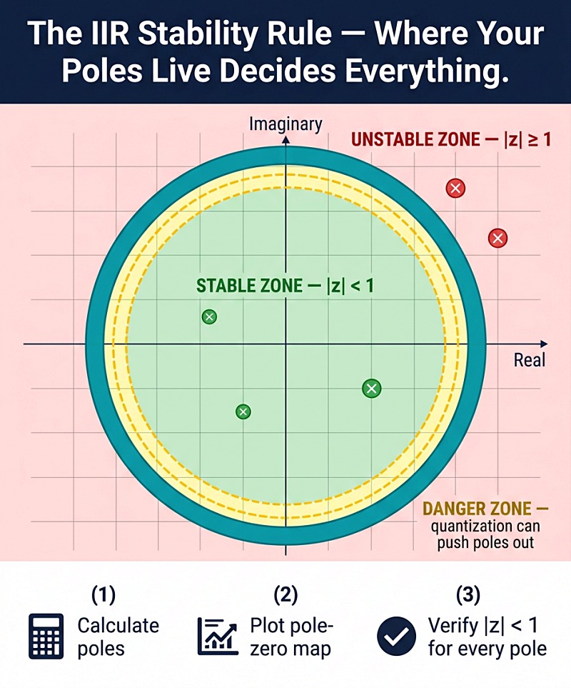
Mathematically, an IIR filter has a transfer function with both numerator and denominator polynomials in z. The roots of the denominator are called poles. According to the bounded-input bounded-output (BIBO) stability criterion documented on Wikipedia, a causal IIR filter is stable if and only if every pole has an absolute value strictly less than one. In plain English: every pole must sit strictly inside the unit circle in the z-plane.

If even one pole touches or crosses that circle, the impulse response no longer decays. It either holds forever (marginal stability, also a failure) or grows without bound (instability). FIR filters do not have this problem because all their poles are at the origin by construction.

That is the textbook answer. The interesting part is why perfectly designed filters still go unstable in real implementations.

How to Tell If Your IIR Filter Is Actually Unstable

Before you start fixing things, confirm the diagnosis. Misdiagnosing a phase issue or an overflow as instability wastes hours.

Run these checks in order:

1. Plot the impulse response. Send a single unit impulse through the filter and graph the output for a few thousand samples. A stable filter decays toward zero. An unstable one grows or oscillates with constant or growing amplitude.
2. Plot the pole-zero map. In MATLAB use zplane(b,a) or pzplot. In Python’s SciPy, use scipy.signal.tf2zpk followed by a polar plot. Every pole must be visibly inside the unit circle.
3. Run an automated stability check. MATLAB’s isstable function from the Signal Processing Toolbox returns 1 if all poles are inside the unit circle and 0 otherwise. SciPy users can check np.all(np.abs(np.roots(a)) < 1).
4. Compute the magnitude of the largest pole. If max(abs(poles)) is anything ≥ 1.0, you have a problem. If it is suspiciously close to 1 (say > 0.99), you have a latent problem that quantization will trigger soon.
5. Test on the actual target hardware. A filter that passes isstable on your dev machine can still blow up on a 16-bit DSP because the coefficients get quantized down. Always test on the deployment platform.

If steps 1-5 confirm instability, move on to the cause table.

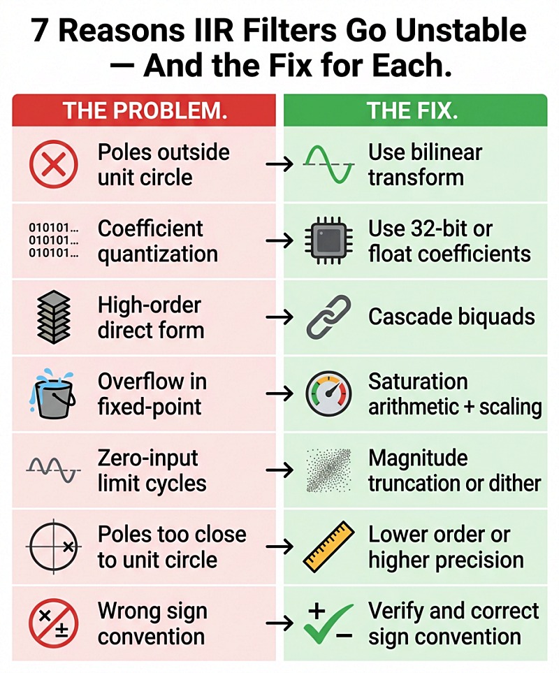
The 7 Real Causes of IIR Filter Instability (Ordered by Frequency)

I have ordered these from most common to least common in real production code. Work the list top down.

1. Poles Outside the Unit Circle (Design-Time Failure)

What happens: The filter design itself produced poles with magnitude ≥ 1. The output grows exponentially.

Why it happens: This usually means you placed poles by hand without checking, used a numerically broken design routine, or transformed an analog prototype using an unsafe method. Direct pole placement, especially for notch and resonator designs, is the common culprit. Old or buggy IIR routines can also produce unstable Butterworth designs at certain orders, as reported on the Scilab users mailing list for Butterworth lowpass at order 4 with low cutoffs.

Fix: Design with the bilinear transform from a known-stable analog prototype (Butterworth, Chebyshev, elliptic). The bilinear transform mathematically guarantees that a stable analog filter maps to a stable digital filter because it maps the entire left half of the s-plane onto the inside of the unit circle in the z-plane. Use battle-tested tools: butter, cheby1, cheby2, ellip in MATLAB or SciPy. Then verify pole magnitudes before deploying anything.

2. Coefficient Quantization Moving Poles Outside (Implementation Failure)

What happens: Your filter is stable in 64-bit floating point but unstable when you convert coefficients to 16-bit fixed point for an MCU or DSP.

Why it happens: Filter coefficients are stored with finite precision. When you round a coefficient like a1 = -1.9876543 to a 16-bit fixed-point value, the actual stored value is slightly different. For poles already close to the unit circle, that tiny coefficient shift can push a pole from radius 0.998 to radius 1.002. The filter is now unstable. This is classically demonstrated in MATLAB’s FDATOOL: a 20th-order elliptic bandpass that is rock-solid in double precision becomes unstable the moment you flip the arithmetic to fixed point.

Fix (in order of effort):

• Use 32-bit or 64-bit coefficients if your platform supports it. Modern Cortex-M4F microcontrollers have hardware floating point and can handle this without breaking a sweat.
• If you must use fixed-point, increase the bit width for both coefficients and state variables to at least 32 bits.
• Decompose the filter into cascaded second-order biquad sections (see cause #3 below) so that quantization affects each pair of poles independently rather than rippling through the whole denominator polynomial.
• For very narrow filters where even biquads struggle, switch to a multirate FIR design or wave digital filter structure.

3. High-Order Direct Form Sensitivity

What happens: Your 4th-order filter works fine. Your 8th-order version goes haywire even at full floating-point precision.

Why it happens: A high-order direct form I or direct form II implementation packs all poles into one big denominator polynomial. The roots of high-order polynomials are extremely sensitive to coefficient changes. This is the famous Wilkinson polynomial problem from numerical analysis: a coefficient change of one part in a million can move the roots by huge amounts. Add quantization on top of that and the filter falls apart.

Fix: Always implement IIR filters of order 3 or higher as a cascade of second-order sections (biquads). MATLAB’s zp2sosor tf2sos and SciPy’s scipy.signal.zpk2sos do this conversion automatically. Each biquad has only two poles and two zeros, so quantization is contained inside that section and cannot ruin the entire response. The ARM CMSIS-DSP library ships production-ready cascaded biquad implementations for exactly this reason.

A typical biquad in transposed direct form II looks like this:

typedef struct {
    float b0, b1, b2, a1, a2;   // Coefficients
    float w1, w2;               // State (delay elements)
} Biquad;

float processBiquad(Biquad *bq, float input) {
    float w0 = input - bq->a1 * bq->w1 - bq->a2 * bq->w2;
    float output = bq->b0 * w0 + bq->b1 * bq->w1 + bq->b2 * bq->w2;
    bq->w2 = bq->w1;
    bq->w1 = w0;
    return output;
}

Cascade as many of these as you need. An 8th-order filter is just four of them in series.

4. Fixed-Point Overflow

What happens: Output looks mostly fine, but you get violent clicks, sudden polarity flips, or the signal wraps from positive max to negative max.

Why it happens: Q15 fixed-point format represents values from roughly -1.0 to +1.0. Inside an IIR filter, intermediate sums can easily exceed that range, especially in resonant or peaking sections where internal gain is much larger than the overall filter gain. When the accumulator wraps around, you get catastrophic glitches that often look like instability but are actually overflow.

Fix:

• Analyze the gain at every node in the filter. Tools like MATLAB’s scale function for SOS structures help with this.
• Apply gain scaling between biquad sections so internal signals stay within range. The classic L-infinity or L2 norm scaling techniques are well documented in any DSP textbook.
• Use saturation arithmetic instead of wraparound. On ARM Cortex-M, the SSAT and USAT instructions clamp to min/max instead of wrapping, which is far less destructive.
• Use a wider accumulator. Q1.31 with a 64-bit accumulator gives you huge headroom inside the math even with Q15 inputs and outputs.
• Easiest of all: switch to floating point if your hardware allows.

5. Zero-Input Limit Cycles

What happens: You feed the filter zero input and instead of going perfectly silent, the output sits at a small constant, or quietly oscillates between a few values forever. Sometimes you can hear it as a faint hum in audio applications.

Why it happens: Quantization is a non-linear operation. Inside an IIR feedback loop, each round of recursion produces a tiny rounding error that gets fed back, multiplied, and rounded again. With certain coefficients, this creates a self-sustaining oscillation that does not decay, even though the linear theory says the filter should be silent. This is exactly the limit cycle problem documented in Analog Devices’ SigmaDSP support knowledge base, where users see persistent post-tone-off output from peak detectors.

Fix:

• Switch to floating-point or higher-precision (32-bit or 64-bit) state variables. Floating point essentially eliminates limit cycles for normal audio and control applications because the rounding error is proportional to the signal magnitude rather than fixed.
• Use magnitude truncation rather than standard rounding for the quantizer in the feedback path. This forces the rounding error to always reduce magnitude, killing the limit cycle.
• Add a small amount of dither noise at the filter input. The decorrelated noise breaks up the periodic pattern that sustains the limit cycle.
• For audiophile applications, use specialized limit-cycle-free structures such as wave digital filters or state-space realizations with proper passivity properties.

6. Poles Too Close to the Unit Circle (Ill-Conditioning)

What happens: Your narrowband bandpass or high-Q resonator works in MATLAB but produces garbage output even with floating-point arithmetic on the host machine. Or it works for one sampling rate but breaks at another.

Why it happens: When you design a filter with a cutoff that is a tiny fraction of the Nyquist frequency (say 1% or less), the poles cluster extremely close to z = 1 (or wherever the band is centered). At that distance from the unit circle, even normal floating-point rounding error during the recursion can momentarily push the effective pole outside, causing transient instability or numerical noise that swamps the desired signal. This is exactly the issue reported on MathWorks Central for Chebyshev Type 2 bandpass filters with low cutoffs at audio sampling rates.

Fix:

• Use the zero-pole-gain (ZPK) representation throughout your design pipeline rather than the transfer function (TF) form. ZPK preserves precision better when poles are clustered.
• Convert to second-order sections (SOS) before implementation. SOS form is far more numerically robust than direct TF form for clustered poles.
• Lower the sample rate (decimate the signal first), apply the filter, then upsample. A filter with a 1% cutoff at 48 kHz becomes a 10% cutoff at 4.8 kHz, with poles much further from the unit circle.
• For extremely narrow filters, consider an FIR alternative or a state-space realization designed specifically to minimize pole sensitivity, as discussed in DSPRelated community threads on narrow IIR designs.

7. Wrong Sign Convention on Feedback Coefficients

What happens: Filter explodes immediately on the first non-zero input, no matter what the design tool said.

Why it happens: This is the dumbest one and it catches everyone at least once. Some libraries use the convention y[n] = b0*x[n] + b1*x[n-1] + ... - a1*y[n-1] - a2*y[n-2] (negative a coefficients in the recursion). Others, including some embedded DSP libraries, use y[n] = b0*x[n] + b1*x[n-1] + ... + a1*y[n-1] + a2*y[n-2] (positive a coefficients, where the negation is already baked into the stored values). If you copy coefficients from a tool that uses one convention into a library that uses the other, the feedback flips sign and the filter goes unstable instantly.

Fix: Read the documentation for the exact filter library you are using. The CMSIS-DSP biquad routines, for example, expect a1 and a2 to be stored already negated. MATLAB’s standard filter function uses the negative convention internally. When in doubt, design a one-pole stable lowpass with a known coefficient (a1 = -0.9), implement it, send a step input, and confirm it settles to the right value before scaling up to your real filter.

How to Fix an Unstable IIR Filter: The Step-by-Step Playbook

Here is the order of operations I follow whenever an IIR filter misbehaves.

Step 1: Confirm the symptom

Plot the impulse response over 5-10 seconds of simulated data. If it grows or sustains, you have instability. If it just sounds wrong but the impulse response decays cleanly, your problem is phase, frequency response shape, or aliasing, not stability.

Step 2: Check the design

Before blaming the implementation, verify that the designed filter is stable in double precision on your host machine. Compute the poles. If max(abs(poles)) >= 1.0, your design tool gave you a bad filter. Redesign using the bilinear transform from a Butterworth or Chebyshev prototype.

Step 3: Convert to second-order sections

Whatever the order, break the filter into biquads using tf2sos (MATLAB) or scipy.signal.tf2sos (Python). Implement using a transposed direct form II or direct form I biquad cascade. This single change fixes the majority of “works on PC, breaks on MCU” cases.

Step 4: Check precision

If you are using fixed point, expand to at least 32-bit coefficients and 32-bit (or 64-bit accumulator) state variables. If you have a hardware FPU, use single-precision float at minimum. For very narrow or high-order filters, use double precision for state even if the I/O is single precision.

Step 5: Add scaling and saturation

Analyze the maximum signal level at every internal node and apply scaling so nothing overflows. Use saturating arithmetic on platforms that support it. For audio, scale headroom of 6-12 dB inside the filter is a safe baseline.

Step 6: Test on the actual target

Run the impulse response test, a long pure-tone test, a zero-input test, and your real-world input on the actual deployment hardware. The host machine and the target almost never behave identically.

Pro Tips Most Tutorials Skip

A few things I learned the hard way that you will not find in the typical first-page articles:

• filtfilt is not magic. It is forward-backward filtering and it doubles your filter order while doing the math twice. With high-Q designs, filtfilt can amplify numerical issues rather than fix them. If filter works but filtfilt blows up, your filter is too steep or too narrow for the precision available.
• Reset your state variables on discontinuities. If your input signal has gaps, level jumps, or sample rate changes, the filter state from “before” can ring through and look like instability. A simple state reset on detected discontinuity often eliminates phantom oscillations.
• Beware the b overflow. Most people scale to prevent overflow at the recursive (a) side but forget that the feedforward (b) coefficients combined with a peaky input can overflow the input section of a Direct Form I biquad. Scale at the input too.
• Cascading order matters. When you cascade biquads, ordering them from lowest-Q (least peaky) to highest-Q section last is often more numerically robust than the opposite. There is no universal best order, but zp2sos in MATLAB has heuristics for this.
• For high-Q resonators, use a state-variable filter. SVF (Chamberlin) topologies are inherently more numerically stable than biquads at high Q with low cutoffs and are the standard in modern audio plugins.

Prevention Checklist

Print this and tape it to your monitor before your next IIR design.

• [ ] Designed using bilinear transform from a stable analog prototype
• [ ] All pole magnitudes verified < 1.0 in double precision
• [ ] Filter order ≥ 3 implemented as cascaded second-order biquads
• [ ] Coefficient bit-width sufficient for pole proximity to unit circle
• [ ] State variables at higher precision than I/O signals
• [ ] Internal scaling analyzed and applied to prevent overflow
• [ ] Saturation arithmetic enabled on fixed-point targets
• [ ] Sign convention of a coefficients matches the target library
• [ ] Impulse response tested on actual deployment hardware
• [ ] Zero-input test confirms no limit cycles
• [ ] Real-input stress test passed at expected signal levels

When to Give Up on IIR and Use FIR Instead

Sometimes the right answer is “do not use an IIR filter for this.” Switch to FIR if any of these apply:

• You need linear phase (audio crossovers, scientific data analysis, communications)
• Your cutoff frequency is below 1% of the sample rate
• You are working with fixed-point hardware where you cannot guarantee enough precision
• The application is safety-critical and you cannot tolerate any possibility of limit cycles or instability

FIR filters are always stable because all their poles are at the origin by construction. The cost is more taps for the same sharpness, which means more compute. With modern hardware, that is rarely a real problem.

FAQ

Why is my IIR filter unstable in MATLAB only when I use fixed-point arithmetic?

Coefficient quantization is the cause. When MATLAB converts your double-precision coefficients to fixed-point format, the rounded values represent slightly different filter poles. If those original poles were close to the unit circle, the quantized poles can land outside it, making the filter unstable. The fix is to use higher coefficient precision, decompose into cascaded biquads (which are far less sensitive to quantization), or accept that very sharp IIR designs may need a multirate FIR alternative.

How do I check if my IIR filter is stable?

Compute the poles of the transfer function (the roots of the denominator polynomial) and check that every pole has magnitude strictly less than 1. In MATLAB, isstable(b,a) returns true if and only if this holds. In Python, use np.all(np.abs(np.roots(a)) < 1). Visually, plot the pole-zero map: every pole must sit inside the unit circle. The closer poles are to the unit circle, the more numerically fragile the filter is, even if it passes the strict stability test.

What causes an IIR filter to oscillate at zero input?

Zero-input limit cycles. They happen because quantization inside the filter’s feedback loop is non-linear. Even when the input is zero, accumulated rounding errors can sustain a small oscillation indefinitely. This is a well-known artifact of fixed-point IIR implementations. The standard fixes are to use floating-point arithmetic, switch the quantizer to magnitude truncation, or add a tiny amount of dither noise to break the periodic pattern.

Are FIR filters always more stable than IIR filters?

Yes. FIR filters have all their poles at the origin (z = 0), so they are unconditionally stable regardless of coefficient values, quantization, or implementation form. IIR filters can be made very stable in practice (cascaded biquads in floating point are essentially bulletproof) but they are never unconditionally stable the way FIR is. If stability matters more than computational efficiency, FIR is the safer default.

Why does cascading biquads improve IIR filter stability?

A high-order IIR filter implemented as one giant direct-form section has a high-order denominator polynomial whose roots are extremely sensitive to coefficient changes. Quantize one coefficient by a tiny amount and any pole can move dramatically. Splitting the filter into cascaded second-order sections means each section has only a quadratic denominator with two poles. Quantization can only move those two poles, not the entire constellation. The result is dramatically better numerical behavior, which is why every production IIR library (CMSIS-DSP, Apple’s Accelerate, Intel IPP, MATLAB DSP System Toolbox) uses cascaded biquads as the default.

Can floating-point IIR filters still be unstable?

Yes, though it is much rarer. Floating-point eliminates most quantization-induced instability, but you can still hit problems with: poles extremely close to the unit circle (sub-1% cutoffs), accumulated round-off in very long-running recursions, very high-order direct-form implementations, and pure design errors where the original pole placement was already unstable. Cascaded biquads in double precision will handle 99% of practical filter designs without issue.

What is the difference between marginal stability and instability?

A marginally stable filter has at least one pole exactly on the unit circle (|z| = 1). The impulse response neither decays nor grows, it sustains forever. In theory it is “not unstable,” but in practice marginal stability is treated the same as instability because any tiny perturbation (quantization, round-off, sample-rate jitter) will tip it over into true instability. A truly stable filter has all poles strictly inside the unit circle (|z| < 1), with reasonable margin.

Should I use Direct Form I or Direct Form II for biquads?

Direct Form I uses more state variables (four per biquad) but is more resistant to overflow because the recursion happens before the gain scaling. Direct Form II uses fewer state variables (two per biquad, hence the memory saving) but can overflow at the internal node before the output saturation can catch it. Transposed Direct Form II is the modern default, used by ARM CMSIS-DSP and most audio libraries: it has Direct Form II’s low memory footprint with much better numerical behavior. Use Transposed DF-II unless you have a specific reason not to.

What to Do Next

If your filter is currently unstable, work the seven causes above in order. Eight times out of ten, the fix is “convert to cascaded biquads and use floating-point coefficients.” If you are designing a new IIR filter, start with the prevention checklist before you write a single line of implementation code.

Bookmark this page. The list of causes does not change, but the temptation to skip the diagnosis steps and start tweaking coefficients does, every single time.